Fundamentals — core workflow

This guide follows one complete path from values in memory to a model you can evaluate. Read it in order the first time; later, use the table of contents to return directly to a concept.

What this guide connects

tensor → Dataset → DataLoader → model → logits → loss
                                      ↓
                         gradients → optimizer update
                                      ↓
                              validation evidence

By the end, you should be able to locate where a batch is created, explain the model's input and output shapes, identify where parameters change, and separate training from evaluation.

Section	Main question	Useful next example
Tensors, shapes, dtype, and device	What does the data mean before it enters a model?	Nonlinear regression
Dataset, transforms, and DataLoader	How do individual samples become batches?	Robust image pipeline
Models, activations, and logits	What contract does an nn.Module provide?	EMNIST classifier
Loss, autograd, and optimizers	How does an error become a weight update?	Training loop
Validation and metrics	How do we check behavior without learning from the check?	Vision and real data

Tensors, shapes, dtype, and device

A tensor is a multidimensional array. Its values are only part of its meaning: shape, dtype, and device are also part of the program.

import torch

x = torch.tensor([[1.0, 2.0], [3.0, 4.0]])
print(x.shape)   # torch.Size([2, 2])
print(x.dtype)   # torch.float32
print(x.device)  # cpu

Read the shape before the layer

Data	Typical shape	Meaning
Tabular batch	[N, F]	samples, features
Image batch	[N, C, H, W]	samples, channels, height, width
Sequence batch	[N, L, E]	samples, sequence length, embedding size
Class logits	[N, K]	samples, classes
Segmentation logits	[N, K, H, W]	samples, classes, spatial prediction

For example, [32, 3, 224, 224] means 32 RGB images at 224 × 224 pixels. The first dimension is the batch; it must survive when features are flattened.

Image tensor reader

Batch Channels Height Width

Reshape without changing the data

x = torch.arange(12).reshape(3, 4)

x.unsqueeze(0).shape       # [1, 3, 4]
x.transpose(0, 1).shape    # [4, 3]
torch.flatten(x).shape      # [12]
torch.flatten(x, 1).shape   # preserves dimension 0 when x is batched

reshape changes how compatible values are viewed; it does not add or remove them. torch.flatten(x, start_dim=1) preserves the batch boundary.

nn.Linear(in_features, out_features) expects the last input dimension to equal in_features:

[N, in_features] × [in_features, out_features] → [N, out_features]

If PyTorch reports mat1 and mat2 shapes cannot be multiplied, print the tensor immediately before the linear layer.

Broadcasting

Broadcasting combines compatible shapes without manually copying data. Dimensions are compared from right to left; each pair must be equal or one must be 1.

batch = torch.ones(4, 3)
bias = torch.tensor([0.1, 0.2, 0.3])
result = batch + bias  # [4, 3]

Broadcasting checker

Shape A Shape B Check shapes

Dtype and device

Neural-network inputs are normally floating point; single-label class targets for CrossEntropyLoss are normally torch.long.

device = torch.device("cuda" if torch.cuda.is_available() else "cpu")
model = model.to(device)
inputs = inputs.to(device=device, dtype=torch.float32)
labels = labels.to(device=device, dtype=torch.long)

The model, inputs, targets, and helper tensors used in the same operation must share a device.

Next: see shape, device, autograd, and nonlinearity together in nonlinear regression.

Dataset, transforms, and DataLoader

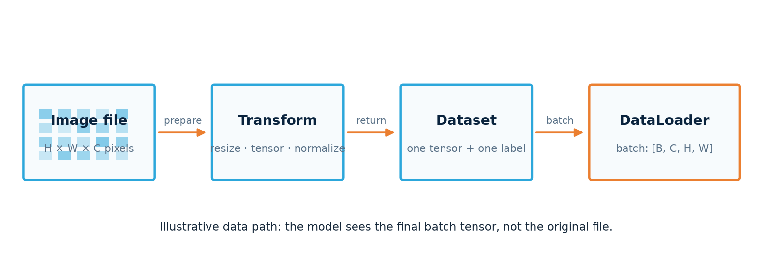
The diagram is structural, not a measured experiment. It shows where a file becomes a tensor and where samples become a batch.

Part	Owns	Produces
Dataset	locating and preparing one valid example	(input, label)
transforms	deterministic preparation or training-only augmentation	a model-ready tensor
DataLoader	batching, order, parallel loading	batches of examples
training loop	device transfer and model updates	loss history and changed parameters

Dataset: one sample

from torch.utils.data import Dataset

class CustomDataset(Dataset):
    def __init__(self, paths, labels, transform=None):
        self.paths = paths
        self.labels = labels
        self.transform = transform

    def __len__(self):
        return len(self.paths)

    def __getitem__(self, index):
        image = load_image(self.paths[index])
        if self.transform:
            image = self.transform(image)
        return image, self.labels[index]

Load lazily in __getitem__; most image projects should not put the complete dataset in memory.

Transforms: prepare consistently

from torchvision import transforms

train_transform = transforms.Compose([
    transforms.RandomHorizontalFlip(),
    transforms.RandomRotation(10),
    transforms.ToTensor(),
    transforms.Normalize(mean, std),
])

validation_transform = transforms.Compose([
    transforms.ToTensor(),
    transforms.Normalize(mean, std),
])

Random, label-preserving augmentation belongs in training only. Validation must be stable between epochs. ToTensor() changes layout to [C, H, W] and normally scales byte pixels to 0–1; normalization is a separate operation.

DataLoader: samples become batches

from torch.utils.data import DataLoader

train_loader = DataLoader(
    train_dataset,
    batch_size=32,
    shuffle=True,
    num_workers=4,
    pin_memory=torch.cuda.is_available(),
)

Batch calculator

Samples Batch size Drop incomplete batch

Inspect one batch before defining the model:

images, labels = next(iter(train_loader))
print(images.shape, images.dtype, images.min(), images.max())
print(labels.shape, labels.dtype, labels.min(), labels.max())

This catches a surprising shape, incorrect label dtype, or wrong class range before a long run.

Next: use the robust image-pipeline project to see validation, corrupt-file reporting, batching, and artifacts together.

Models, activations, and logits

An nn.Module owns trainable layers and defines how an input becomes an output.

from torch import nn

class Classifier(nn.Module):
    def __init__(self, input_features: int, classes: int):
        super().__init__()
        self.network = nn.Sequential(
            nn.Linear(input_features, 128),
            nn.ReLU(),
            nn.Linear(128, classes),
        )

    def forward(self, x):
        return self.network(x)  # [batch, classes]

• __init__ creates reusable layers and registers their parameters.
• forward describes the transformation.
• model(x) is the normal call; it preserves hooks and PyTorch internals.
• The output is raw logits, one score per class.

Why activations matter

linear = nn.Linear(1, 1)

nonlinear = nn.Sequential(
    nn.Linear(1, 32),
    nn.Tanh(),
    nn.Linear(32, 1),
)

Stacking only linear layers remains a linear transformation. An activation such as ReLU or Tanh lets the network represent bends and nonlinear decision boundaries.

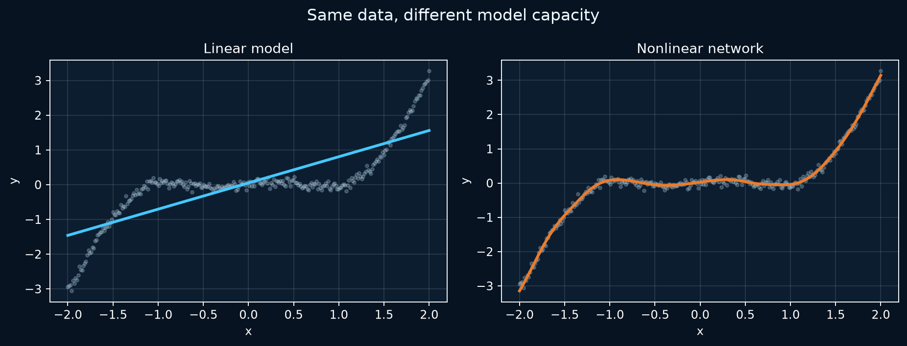
This chart is reproduced by the retained regression script with a fixed seed. It demonstrates model capacity, not a general benchmark.

Logits, probabilities, and predictions

For single-label multiclass classification:

logits = model(inputs)                 # [batch, classes]
loss = nn.CrossEntropyLoss()(logits, labels)
predictions = logits.argmax(dim=1)    # [batch]
probabilities = logits.softmax(dim=1) # only when probabilities are needed

Do not apply softmax before CrossEntropyLoss; the loss already combines the stable operations it needs.

Next: the EMNIST project compares a dense classifier with a CNN and produces predictions, curves, metrics, and a checkpoint.

Loss, autograd, and optimizers

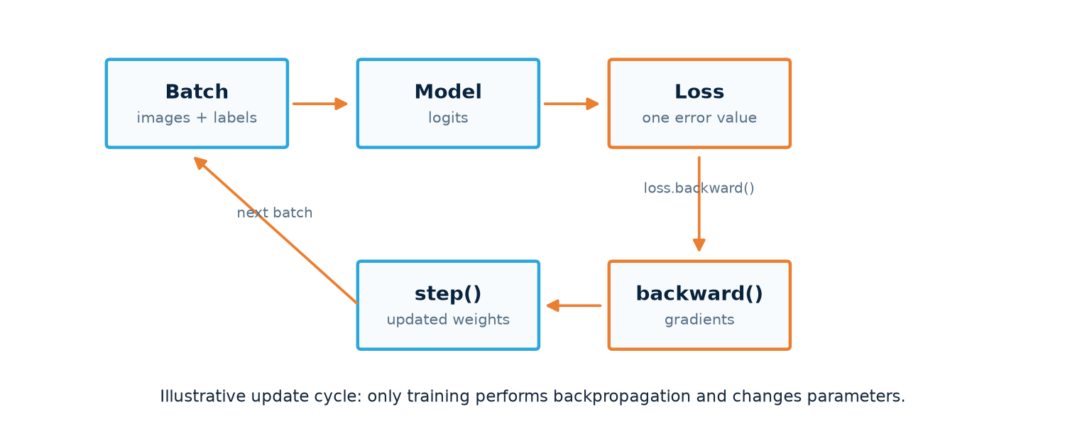
Loss turns model behavior into one differentiable scalar. Autograd follows the operations that produced it, and the optimizer uses the resulting gradients to update parameters.

w = torch.tensor(2.0, requires_grad=True)
x = torch.tensor(3.0)
y = (w * x) ** 2
y.backward()
print(w.grad)

Gradients accumulate by default. That is why each independent update clears old gradients before backpropagation.

The complete training loop

Training-loop stepper

1. Clear old gradients
2. Run the forward pass
3. Measure the loss
4. Backpropagate gradients
5. Update parameters

Previous Next

def train_epoch(model, loader, loss_fn, optimizer, device):
    model.train()
    total_loss = 0.0

    for inputs, labels in loader:
        inputs = inputs.to(device)
        labels = labels.to(device)

        optimizer.zero_grad(set_to_none=True)
        logits = model(inputs)
        loss = loss_fn(logits, labels)
        loss.backward()
        optimizer.step()

        total_loss += loss.item() * inputs.size(0)

    return total_loss / len(loader.dataset)

Step	Reads	Changes
zero_grad()	optimizer parameter list	clears stored gradients
model(inputs)	inputs and parameters	creates activations and the computation graph
loss_fn(...)	logits and targets	creates the scalar objective
loss.backward()	computation graph	accumulates parameter gradients
optimizer.step()	parameters and gradients	updates parameters

optimizer = torch.optim.Adam(model.parameters(), lr=1e-3)

A learning rate that is too high can make loss unstable; one that is too low can make progress impractically slow. Before a full run, try to overfit one small batch. If loss cannot fall, inspect labels, loss pairing, gradients, and optimizer ownership.

Advanced variations keep this basic order: gradient clipping goes after backward() and before step(); accumulation delays step(); mixed precision wraps the forward/loss work and scales gradients.

Validation and metrics

Evaluation uses the same model without updating its parameters.

def evaluate(model, loader, device):
    model.eval()
    correct = 0
    total = 0

    with torch.no_grad():
        for inputs, labels in loader:
            inputs = inputs.to(device)
            labels = labels.to(device)
            logits = model(inputs)
            predictions = logits.argmax(dim=1)
            correct += (predictions == labels).sum().item()
            total += labels.size(0)

    return correct / total

model.eval() changes dropout and batch-normalization behavior. torch.no_grad() disables gradient tracking and reduces memory use. Use both; neither computes a metric by itself.

Choose evidence for the question

Metric	Useful when	Limitation
Accuracy	classes are reasonably balanced	can hide minority-class failure
Precision	false positives are costly	ignores missed positives
Recall	false negatives are costly	ignores false alarms
F1	precision and recall both matter	averages can hide class-specific failure
Confusion matrix	you need the structure of mistakes	requires inspection, not one scalar

Weight epoch loss by sample count so a smaller final batch does not count like a full batch:

running_loss += loss.item() * inputs.size(0)
epoch_loss = running_loss / len(loader.dataset)

Prevent leakage

• Split before fitting data-dependent preprocessing.
• Keep class-to-index mapping identical across splits.
• Do not apply random training augmentation to validation.
• Tune with validation, not repeatedly with the final test set.
• Select a checkpoint using validation behavior; evaluate on test once.

Core-workflow checklist

Before trusting a run, answer these questions:

1. What does each input dimension mean?
2. Are input, target, and parameters on the same device?
3. Does the Dataset return one valid sample and label?
4. Do model outputs have shape [batch, classes]?
5. Does the loss match the output and target representation?
6. Are gradients cleared, calculated, and applied in the intended order?
7. Does evaluation use stable data, eval(), and no gradients?
8. Can the pipeline overfit one tiny batch?

Continue with Fundamentals — vision and real data, where the same workflow is applied to images, CNNs, imperfect files, and generalization.