Fundamentals — vision and real data

This guide applies the core PyTorch workflow to image data. It connects convolution, changing tensor shapes, reliable input pipelines, generalization, and model saving into one practical sequence.

What this guide connects

image files → validated samples → augmented training batches
                                      ↓
                         convolutional feature maps
                                      ↓
                           [batch, classes] logits
                                      ↓
                 validation curves + error inspection
                                      ↓
                    reproducible checkpoint and context

Read Fundamentals — core workflow first if Dataset, logits, loss, or the training update order are unfamiliar.

Section	Main question	Useful next example
Convolution and feature maps	How does a CNN look for local patterns?	EMNIST
CNN architecture and shapes	Where do channels grow and spatial dimensions shrink?	Nature CNN
Reliable image data	What must be true before a metric is trustworthy?	Robust pipeline
Generalization and regularization	Is the model learning a reusable pattern or memorizing?	Learning curves
Saving and restoring	What must be retained to use the model again?	Reference

Convolution and feature maps

A dense layer sees one long list of pixels. A convolution keeps the spatial layout and applies the same small kernel at many positions. Reusing weights makes it efficient and allows one learned pattern to be recognized in different locations.

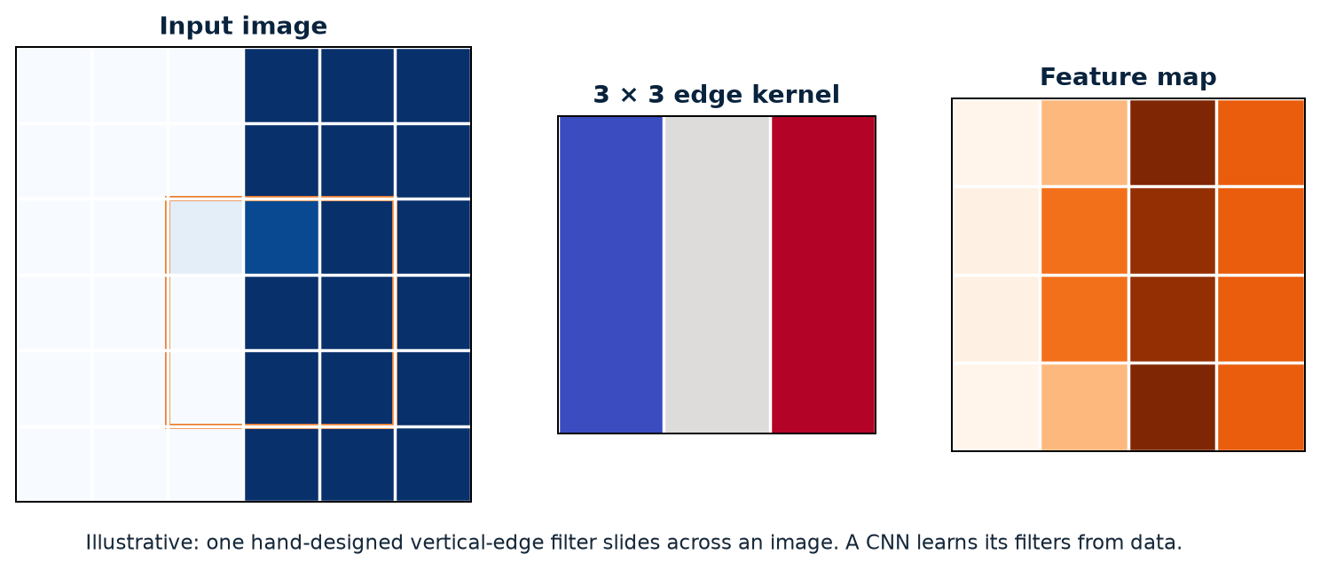
The pictured filter is hand-designed to make its response visible. A trained CNN learns its kernel values through backpropagation.

3 × 3 kernel explorer

Kernel Vertical edge Horizontal edge Sharpen Box blur Randomize input

Input

Kernel

Valid output

Channels

nn.Conv2d(
    in_channels=3,
    out_channels=32,
    kernel_size=3,
    padding=1,
)

Each of the 32 learned filters spans all three RGB input channels. The result is 32 feature maps—not 32 colours. Early filters may respond to edges, colour transitions, or texture; deeper layers combine those maps into patterns useful for the task.

Kernel size, stride, and padding

• Kernel size controls the local window inspected at once.
• Stride controls how far the kernel moves between positions.
• Padding adds a border so edge pixels participate and output size can be controlled.
• Dilation spaces kernel elements apart to expand the receptive field.

For one spatial dimension:

output = floor((input + 2 × padding − dilation × (kernel − 1) − 1) / stride + 1)

A 3 × 3 convolution with padding 1, stride 1, and dilation 1 preserves height and width.

CNN architecture and shapes

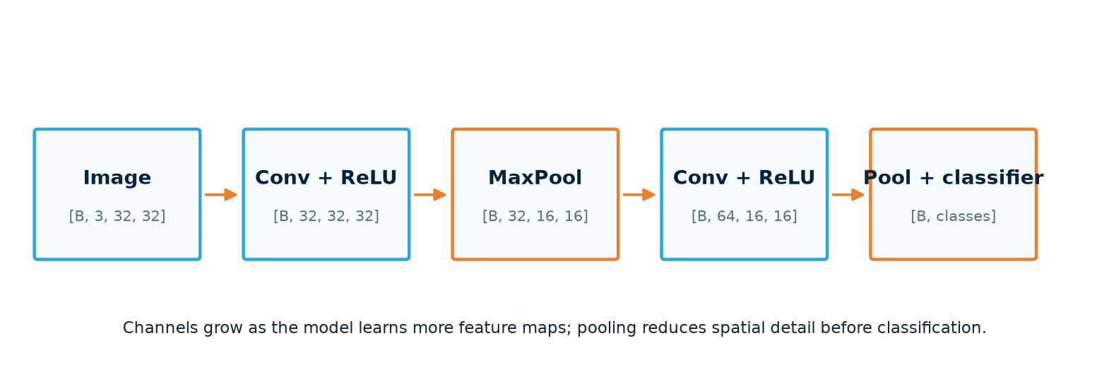
The values in the diagram are an illustrative shape trace. Always inspect the real input and real model.

[batch, 3, 32, 32]
  → convolution: channels grow
  → pooling or stride: width and height shrink
  → classifier: [batch, classes]

A reusable block

class CNNBlock(nn.Module):
    def __init__(self, in_channels, out_channels):
        super().__init__()
        self.block = nn.Sequential(
            nn.Conv2d(in_channels, out_channels, 3, padding=1),
            nn.BatchNorm2d(out_channels),
            nn.ReLU(),
            nn.MaxPool2d(2),
        )

    def forward(self, x):
        return self.block(x)

Convolution learns local features, ReLU adds nonlinearity, normalization stabilizes intermediate distributions, and pooling reduces spatial resolution.

CNN shape tracer

Input size Pooling blocks Trace

Safer classifier boundaries

Hard-coded flatten sizes break when input resolution or feature blocks change. Prefer adaptive pooling when spatial position no longer needs to be preserved:

self.features = nn.Sequential(
    CNNBlock(3, 32),
    CNNBlock(32, 64),
    nn.AdaptiveAvgPool2d((1, 1)),
)
self.classifier = nn.Linear(64, classes)

def forward(self, x):
    x = self.features(x)
    x = torch.flatten(x, 1)
    return self.classifier(x)

When a fixed feature size is intentional, inspect it with a dummy input rather than calculating it mentally:

with torch.no_grad():
    features = self.features(torch.zeros(1, 3, 32, 32))
print(features.shape)

Trace the first unexpected shape

def show_shape(name):
    def hook(module, inputs, output):
        print(name, tuple(output.shape))
    return hook

handle = model.features.register_forward_hook(show_shape("features"))
# run one batch, then remove the temporary hook
handle.remove()

Most shape failures are easier to understand at the first incorrect boundary than at the final linear-layer error.

Next: compare a dense model with a CNN in EMNIST, then inspect a modular regularized model in Nature CNN.

Reliable image data

A larger architecture cannot repair inconsistent labels, leakage, corrupt files, or transforms applied to the wrong split.

Establish the data contract before training

1. Define stable class names and a class-to-index mapping.
2. Verify file existence, extension, readability, colour mode, and expected input shape.
3. Record rejected files with their path and reason.
4. Split with a fixed seed before applying random augmentation.
5. Inspect class counts in each split.
6. Keep validation preprocessing deterministic.
7. Split related entities together so near-duplicates cannot leak across sets.

from PIL import Image

def open_rgb(path):
    with Image.open(path) as image:
        return image.convert("RGB")

Handle failures deliberately

Do not recursively request another sample from __getitem__ without a strict limit; a cluster of corrupt files can create infinite recursion. Prefer validating the index before training. When runtime filtering is required, return a controlled sentinel and use a custom collate_fn.

def collate_valid(batch):
    valid = [sample for sample in batch if sample is not None]
    if not valid:
        raise RuntimeError("Batch contains no valid samples")
    return torch.utils.data.default_collate(valid)

Make splits reproducible

generator = torch.Generator().manual_seed(42)
train_set, validation_set = random_split(
    dataset,
    [train_size, validation_size],
    generator=generator,
)

Record the split seed and per-class distribution. For multiple images of the same person, object, location, or capture burst, split by entity rather than individual image.

Monitor data, not only the model

• Samples and rejected files per class.
• Pixel range after transforms.
• Label dtype and minimum/maximum values.
• Batch loading time and accelerator idle time.
• Class mapping stored with the run.
• Example transformed images from both training and validation.

The robust image-pipeline project downloads public data, builds a folder dataset, adds one known corrupt file, records the validation decision, and trains only on valid examples.

Generalization and regularization

Generalization asks whether patterns learned from training examples remain useful on unseen data from the intended environment.

Read learning curves

Learning-curve comparison

Illustrative regularization strength

Illustrative curves—not measured benchmark results.

Observation	Likely issue	First checks
Training and validation both poor	underfitting or broken pipeline	labels, loss, learning rate, capacity
Training improves; validation worsens	overfitting	split quality, augmentation, regularization
Loss becomes NaN	numerical instability	invalid inputs, learning rate, gradients
High total accuracy; one class fails	imbalance or shortcut learning	per-class recall and confusion matrix

Four gaps to inspect

1. Training–validation gap: has the model fitted training-specific detail?
2. Validation–deployment gap: does validation represent real inputs?
3. Aggregate–class gap: does one headline metric hide weak classes?
4. Accuracy–cost gap: is an improvement worth the memory, latency, and complexity?

A model can improve on a standard held-out set and still fail on an external source. Report both domains instead of treating one as the universal truth.

Regularization tools

Data augmentation creates realistic label-preserving variation. An upside-down vehicle or severely distorted character may not preserve the label.

Weight decay discourages unnecessarily large weights:

optimizer = torch.optim.AdamW(
    model.parameters(),
    lr=1e-3,
    weight_decay=1e-4,
)

Dropout randomly removes activations during training:

self.dropout = nn.Dropout(0.3)

It is active in model.train() and disabled in model.eval().

Early stopping keeps the checkpoint associated with the best validation behavior instead of assuming the final epoch is best.

Change one hypothesis at a time. Use the same split, seed, metrics, and evaluation procedure so an apparent gain does not come from changing the test.

Saving and restoring

Save model parameters

torch.save(model.state_dict(), "model.pth")

Restore them into the same architecture:

model = Classifier(classes=len(class_names))
state = torch.load("model.pth", map_location=device, weights_only=True)
model.load_state_dict(state)
model.to(device)
model.eval()

Save a training checkpoint

torch.save({
    "epoch": epoch,
    "model_state": model.state_dict(),
    "optimizer_state": optimizer.state_dict(),
    "validation_loss": validation_loss,
    "class_names": class_names,
    "input_shape": input_shape,
    "normalization": normalization,
}, "checkpoint.pth")

A usable model is more than its tensors. Retain architecture code, preprocessing, class order, input shape, selected metric, split identity, seed, and package versions. Verify the restored model on a known input.

Never load an untrusted pickle-based checkpoint. Prefer weight-only loading when the saved format and installed PyTorch version support it.

Vision-workflow checklist

Before trusting an image model, confirm:

1. Files, labels, classes, and splits were validated before training.
2. Training and validation transforms differ only where intended.
3. Every CNN boundary has a known shape.
4. The classifier produces [batch, classes] logits.
5. Metrics include error structure, not only one average.
6. Training and validation curves are interpreted together.
7. The selected checkpoint can be restored with its preprocessing and class order.

Use the project gallery to move from these patterns to complete, runnable examples, or open the reference when debugging a specific run.