Training — metrics and tuning

Once the basic training loop works, the question changes: which settings improve the result, and what evidence makes the comparison fair?

Read in order: choose a metric → establish a baseline → tune the learning rate → schedule it → search a few settings → compare quality and cost. For faster execution of the same experiment, continue with efficient training.

Code key: “Runnable toy” includes imports and inputs. Other snippets are excerpts: reuse torch, nn, and the model, loader, tokenizer or helper named in the section. Projects contain the complete runnable scripts.

Metrics that answer the right question

Inspection outcomes → metrics

Positive means “defect”. Rows are truth; columns are predictions.

True positives False positives False negatives True negatives

Try always predicting “good”

Exact arithmetic on editable counts; no trained detector.

The loss is the differentiable quantity used to train. A metric describes behavior you care about. Lower cross-entropy and higher accuracy often move together, but they are different measurements.

For one positive class, imagine an inspection system:

Outcome	Meaning
TP	a defect was correctly flagged
FP	a good item was flagged
FN	a defect was missed
TN	a good item was correctly accepted

accuracy  = (TP + TN) / all samples
precision = TP / (TP + FP)        how trustworthy are the alarms?
recall    = TP / (TP + FN)        how many defects did we find?
F1        = 2 × precision × recall / (precision + recall)

If 99 of 100 items are good, always predicting “good” gives 99% accuracy and zero defect recall. F1 does not include true negatives, and no metric removes the need to inspect actual mistakes. A confusion matrix shows which classes get confused; state whether rows represent true or predicted classes.

Average over the dataset

In multiclass work, macro gives every class equal weight; weighted weights classes by support; micro pools the underlying counts. For ordinary single-label multiclass predictions over all classes, micro precision, recall and F1 equal accuracy. Macro F1 is the average of per-class F1 values, not F1 calculated from macro precision and recall.

Code and details

This excerpt needs TorchMetrics, an existing model, validation loader and device:

from torchmetrics.classification import MulticlassF1Score

metric = MulticlassF1Score(num_classes=classes, average="macro").to(device)
model.eval()
with torch.no_grad():
    for x, y in validation_loader:
        logits = model(x.to(device))
        metric.update(logits.argmax(1), y.to(device))
macro_f1 = metric.compute().item()
metric.reset()  # do this before measuring the next epoch with the same object

Use MulticlassAccuracy, MulticlassPrecision, MulticlassRecall and MulticlassConfusionMatrix similarly. update() accumulates counts; compute() summarizes them; reset() starts a new measurement. Averaging individual batch F1 values is generally incorrect. Keep separate state for training and validation.

What each hyperparameter changes

Parameters are learned weights and biases. Hyperparameters are choices you set around that learning process.

Choice	What changes	Watch for
lr	size of optimizer updates	divergence when high; slow learning when low
optimizer	update rule: SGD, momentum, Adam/AdamW	each rule needs its own LR comparison
batch_size	samples per update, memory and gradient variability	more throughput does not guarantee better validation
epochs	data passes / training budget	the final epoch may overfit
blocks / channels / hidden width	representation capacity and compute	more layers can shrink images too far
kernel size	spatial window per convolution	padding and feature shapes must remain valid
dropout p	fraction of activations dropped during training	excessive dropout can cause underfitting
weight_decay	pressure against large weights	AdamW decouples it from the adaptive gradient update
BatchNorm	learned scaling plus running statistics	behavior depends on training mode and microbatch size
early stopping patience	how long to wait without useful improvement	counts validation checks, not universally epochs

Try a small logarithmic LR range first, for example 1e-4, 1e-3, 1e-2. These are experiment candidates, not universal defaults. Compare the same split, initialization policy, training budget and metric. Change one hypothesis at a time before widening the search.

Learning-rate schedulers

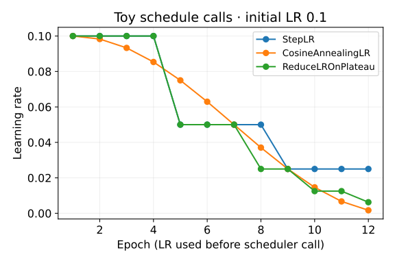
Toy execution: StepLR halves LR every four calls; cosine spans 12 epochs; plateau responds to the declared validation-loss signal [1, .8, .8, .8, .7, .7, .7, .7, .7, .7, .7, .7] with patience 1. The chart shows LR used before each end-of-epoch scheduler call. This is a schedule comparison, not measured model training. Calls and values.

StepLR0.001 → 0.0005 → 0.00025drop after every 4 epoch calls

Cosinehigh → smooth lowT_max counts schedule calls

Plateauvalidate → compare → maybe reducepatience waits for non-improving checks

Illustrative schedules. A short improving run may never trigger a plateau reduction. Log LR used before the step and LR next afterward.

An optimizer changes weights; a scheduler changes the optimizer's LR. It cannot repair wrong labels or leakage.

Scheduler	Key parameters	Call it…
StepLR	step_size, gamma	after updates at each chosen interval
CosineAnnealingLR	T_max, eta_min	after updates; T_max counts scheduler calls
ReduceLROnPlateau	mode, factor, patience, threshold	after validation with the monitored value

For an epoch-based schedule:

optimizer = torch.optim.AdamW(model.parameters(), lr=1e-3)
scheduler = torch.optim.lr_scheduler.StepLR(optimizer, step_size=4, gamma=0.5)
for epoch in range(epochs):
    train_epoch(model, train_loader, loss_fn, optimizer, device)
    validation_loss = validate_epoch(model, validation_loader)
    used_lr = optimizer.param_groups[0]["lr"]
    scheduler.step()  # changes the rate for the next epoch

Here train_epoch and validate_epoch are your training/evaluation functions. With this schedule, the first four epochs use 1e-3, the next four 5e-4, then 2.5e-4. get_last_lr() returns the scheduler's latest rates; logging before or after the step describes different epochs.

Plateau scheduling needs a matching direction:

scheduler = torch.optim.lr_scheduler.ReduceLROnPlateau(
    optimizer, mode="min", factor=0.5, patience=2,
)
scheduler.step(validation_loss)  # once after each validation measurement
# For accuracy/F1 instead: mode="max", then step(validation_score).

Common trap: changing an epoch-based call to every batch silently speeds up the schedule. Early stopping and plateau scheduling also have different jobs: one ends training; the other lowers LR and continues.

A small Optuna search

Trial: one proposed configuration and its measurement. Objective: your function that trains/evaluates that configuration and returns a scalar. Study: the collection of trials and its optimization direction.

The structure below requires Optuna and your own fit_and_validate function. Each call must build a fresh model and optimizer, use the same data split, and return validation macro F1:

Implementation excerpt · requires the objects described above

import optuna

def objective(trial):
    settings = {
        "lr": trial.suggest_float("lr", 1e-4, 1e-2, log=True),
        "width": trial.suggest_int("width", 16, 64, step=16),
        "dropout": trial.suggest_float("dropout", 0.0, 0.4),
        "kernel": trial.suggest_categorical("kernel", [3, 5]),
    }
    score, seconds = fit_and_validate(settings)
    trial.set_user_attr("training_seconds", seconds)
    return score

study = optuna.create_study(
    direction="maximize", sampler=optuna.samplers.TPESampler(seed=17),
)
study.optimize(objective, n_trials=12)
print(study.best_params, study.best_value)
table = study.trials_dataframe()

suggest_int chooses discrete integers; suggest_float(log=True) searches orders of magnitude; suggest_categorical chooses named options. If the objective is loss, use direction="minimize".

Grid search exhausts listed combinations; random search samples without learning from scores; TPE uses earlier trials to guide later proposals. A short search has noisy evidence. optuna.visualization.plot_optimization_history(study), plot_param_importances(study) and plot_parallel_coordinate(study) help explore completed trials; their plotting dependencies are optional. Those plots do not establish causation or a global optimum. Recheck promising settings across seeds.

Flexible models must register every layer

Use nn.Sequential(*blocks) for an ordered chain or nn.ModuleList(blocks) when your forward chooses how to use registered blocks. A plain Python list does not register layers with the parent model.

If a classifier is created on its first forward pass, run a representative dummy input before constructing the optimizer, with the model on the intended device. Otherwise the optimizer can miss those new parameters. Prefer constructing the head in __init__ using adaptive pooling when practical. Model inspection makes registration visible.

Quality within a budget

Compare validation quality with trainable parameter count, parameter/buffer bytes, peak training memory, and inference latency. They answer different questions. See measurement code.

Apply hard limits first: discard models that exceed required memory or latency, then choose among the feasible candidates. For flexible priorities, normalize metrics to comparable scales and invert costs before a weighted sum. The chosen weights encode your priorities; scores can change when the candidate set changes. Avoid repeatedly testing every candidate on the final test set.

Remember and apply

Check yourself: validation macro F1 improves but latency violates the device limit. Is the new model better for that deployment? It fails a required constraint, even though its classification score improved.

Record configuration, split identity, seed, packages, validation results, time and memory. Select the checkpoint using validation, then perform the final test evaluation. Continue with efficient training to measure where the run spends its resources.

Run the idea: Controlled training comparison combines the same initial weights and split, two learning rates, macro F1, plateau scheduling and gradient accumulation in one small original script.

Sources: TorchMetrics classification, PyTorch schedulers, Optuna trials and studies.