Vision — data, transforms and noise

An image model learns from the tensors it receives, not the files you intended to give it. TorchVision connects loading, datasets, transformations and visual inspection.

Build on images and CNNs. This page explains the inputs; pretrained vision models explains what to do with them.

Code key: “Runnable toy” includes imports and inputs. Other snippets are excerpts: reuse torch, nn, and the model, loader, tokenizer or helper named in the section. Projects contain the complete runnable scripts.

PIL, tensors and image utilities

Representation / function	Meaning
PIL image.size	(width, height); check mode such as RGB/L/RGBA
decode_image(path)	normally byte tensor [C,H,W], often uint8 in 0..255
transforms.ToTensor()	typical byte/PIL input → floating [C,H,W] in 0..1
ToPILImage()	converts a supported tensor/array for PIL use
make_grid(batch, nrow=...)	combines equal-size [N,C,H,W] images for inspection
save_image(tensor, path)	saves a display-ready float image/grid

from PIL import Image
from torchvision import transforms
from torchvision.utils import make_grid, save_image
import torch

with Image.open("sample.jpg") as image:
    rgb = image.convert("RGB")
prepared = transforms.Compose([
    transforms.Resize(256), transforms.CenterCrop(224), transforms.ToTensor(),
])(rgb)
grid = make_grid(torch.stack([prepared, prepared.flip(-1)]), nrow=2)
save_image(grid, "inspection.png")

Use your own image path. Resize(256) preserves aspect ratio and makes the shorter side 256; Resize((256,256)) forces a square and can distort it. CenterCrop(224) gives a consistent shape but can remove an off-centre object. ToTensor() scaling depends on input type; it is not a generic “divide every array by 255” rule.

Choose a dataset interface

Tool	Use	Important detail
MNIST / FashionMNIST	grayscale image-classification baselines	[1,28,28] before batching
CIFAR10 / CIFAR100	small RGB classification benchmarks	different class counts
EMNIST	digits / letters and other splits	choose split; Letters labels begin at 1
SVHN	house-number digit images	uses split="train" / "test"
OxfordIIITPet / Flowers102	specialized image data	examine each dataset's labels and split interface
ImageFolder(root)	your images in class subfolders	class mapping derives from directory names
FakeData(...)	generated images/labels for code checks	meaningless labels for a quality benchmark
custom Dataset	CSV, separate labels, special validation	explicitly define sample/label contract

Detection, segmentation, video, captioning and optical-flow datasets have different targets. Do not assume every dataset returns a single integer class.

With ImageFolder, inspect .classes, .class_to_idx and one sample before training. Confirm training and validation mappings match. With EMNIST Letters, map labels 1..26 to 0..25 for cross-entropy and verify image orientation against displayed samples. Fixed orientation correction is preprocessing, not random augmentation.

random_split returns subsets referring to the same underlying dataset. Setting train_subset.dataset.transform can therefore also change validation. Use separate dataset objects with the same split indices, or a per-subset transform wrapper. See the split example.

Build the transform pipeline in order

Same original target through actual TorchVision transforms; seed 71. Variation is for inspection, not a model-quality result.

PIL RGB(width,height); bytes 0..255spatial and color augmentation

ToTensor[3,H,W]; float 0..1add tensor noise here

Normalize(x − mean) / stdnegative values are normal

Displayx × std + meanreverse normalization before viewing

Illustration: shapes and operations, not measured model performance.

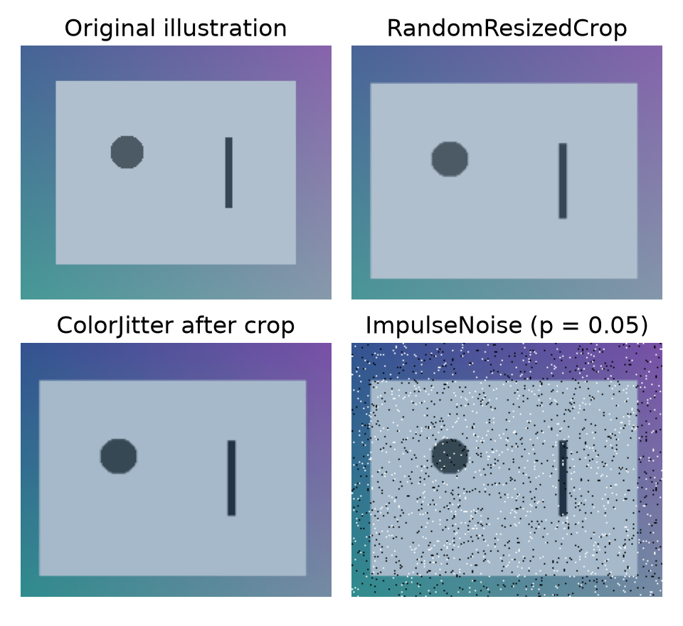
In the saved panel execution, the PIL scene is 220×180 RGB. ToTensor produces [3,180,220] in [0,1]; normalization with mean/std 0.5/0.5 keeps that shape and maps the observed range to [-1,1]. Reverse it with x * 0.5 + 0.5 for display. These are the toy panel's settings, not every pretrained model's required normalization.

Preprocessing makes inputs compatible. Augmentation exposes training to plausible variation. Most random transforms sample a new version when a sample is accessed; they do not permanently multiply files on disk.

open RGB → spatial changes → pixel changes → float tensor → noise → normalize

Transform	Parameters to remember	Use carefully because…
RandomResizedCrop	size, scale, ratio	a crop may discard the label-defining feature
RandomHorizontalFlip	probability p	text/symbols and some asymmetric objects change meaning
RandomRotation	degree range	rotation may introduce fill borders
RandomAffine	degrees, translate, scale, shear	geometric distortion must reflect plausible inputs
ColorJitter	brightness, contrast, saturation, hue	colour may be essential to the class
RandomApply	transforms and p	controls whether a group is applied
custom callable	__call__ input/output contract	order depends on PIL vs tensor representation

For a scratch RGB classifier, after selecting training-only statistics:

# ImpulseNoise is the original tensor transform shown below.
train_transform = transforms.Compose([
    transforms.RandomResizedCrop(96, scale=(0.8, 1.0)),
    transforms.RandomHorizontalFlip(p=0.5),
    transforms.ColorJitter(brightness=0.15, contrast=0.15),
    transforms.ToTensor(),
    ImpulseNoise(amount=0.01),
    transforms.Normalize(mean, std),
])
validation_transform = transforms.Compose([
    transforms.Resize(112), transforms.CenterCrop(96),
    transforms.ToTensor(), transforms.Normalize(mean, std),
])

The crop size and noise amount are illustrative choices. A pretrained model should instead use its weight-specific preprocessing contract. Start mildly, display repeated versions of the same sample, and compare validation with a no-augmentation baseline.

Noise as a controlled augmentation

The studied lab implements salt and pepper noise: scattered bright and dark pixels. The idea is to expose a classifier to some corruption while preserving the class. It is a custom transform, not a learned denoiser.

Noise / degradation	Appearance	Interpretation
Salt and pepper / impulse	isolated white or black pixels	an approximation to impulse-like corruption or faulty pixels
Gaussian, an extra comparison here	small additive fluctuations	a simplified model of some read-noise behavior
Shot noise, conceptual extension	variability depends on intensity	photon statistics are signal-dependent
Blur, brightness, compression	different spatial/tonal defects	not interchangeable with random pixel noise

The lab's implemented example is impulse noise. Gaussian and shot noise are included here to distinguish mechanisms, not as additional lab experiments. Real cameras combine exposure, gain, photon noise, readout, processing and potentially fixed patterns. Synthetic noise alone does not predict a camera's performance.

See the corruption, keep the scene

Noise Salt and pepperGaussian comparison Amount

Clean synthetic target

Corrupted target

Salt and pepper: 5% of spatial pixels selected in expectation.

Seeded illustrative pixels; no trained model, camera measurement or accuracy prediction.

An original tensor transform

This transform expects a floating [C,H,W] image in [0,1]. Apply it after ToTensor() and before Normalize():

Code and details

class ImpulseNoise:
    """Replace selected spatial pixels in a float [C,H,W] image in [0,1]."""
    def __init__(self, amount=0.02, salt_fraction=0.5):
        if not 0 <= amount <= 1 or not 0 <= salt_fraction <= 1:
            raise ValueError("Noise probabilities must be in [0, 1]")
        self.amount = amount
        self.salt_fraction = salt_fraction

    def __call__(self, image):
        # One mask shared across channels: a selected RGB pixel is white or black.
        draw = torch.rand_like(image[:1])
        salt = draw < self.amount * self.salt_fraction
        pepper = (draw >= self.amount * self.salt_fraction) & (draw < self.amount)
        noisy = torch.where(salt, torch.ones_like(image), image)
        return torch.where(pepper, torch.zeros_like(image), noisy)

Use import torch. amount=0.02 selects approximately 2% of spatial pixels; salt_fraction=0.5 splits selected pixels equally between bright and dark in expectation. Every channel of a selected RGB pixel is changed together. Selection is probabilistic, so the exact number varies. The input is preserved and edge pixels participate too.

For the additional Gaussian comparison, an original one-line mechanism is (image + sigma * torch.randn_like(image)).clamp(0, 1). sigma is measured in the pre-normalization pixel scale; 0.03 means a standard deviation of 3% of that full range. Clipping changes the resulting distribution at black and white.

Common trap: adding [0,1] noise to already normalized pixels then clipping to [0,1] destroys the normalized input. Another trap is using such strong noise that the label can no longer be inferred.

Keep ordinary validation deterministic. If you need a corruption robustness test, define a separate fixed-seed/fixed-severity evaluation and report it alongside clean validation, not mixed into a fluctuating metric.

Normalization and display

For each channel, Normalize(mean, std) applies (pixel - mean) / std. It does not guarantee a Gaussian distribution and does not clamp to [0,1]. Negative normalized values are normal.

For a scratch model, estimate statistics from the training split, using deterministic preprocessing and no random noise. Across channel values, accumulate sum, sum of squares and the actual pixel count:

mean = sum / count
variance = sum_of_squares / count - mean²
std = sqrt(max(variance, 0))

Use stable accumulation, guard against zero standard deviation, and keep the resulting constants for validation/test. Averaging image standard deviations does not generally equal the global pixel standard deviation.

For display, reverse normalization first:

mean_tensor = torch.tensor(mean, device=image.device)[:, None, None]
std_tensor = torch.tensor(std, device=image.device)[:, None, None]
display_image = (image * std_tensor + mean_tensor).clamp(0, 1)

make_grid(normalize=True) rescales a visualization; it is not the same operation as training normalization and can hide a bad pixel range. Inspect numeric values as well as the picture.

Remember and apply

Check yourself: a flip makes a symbol look like a different symbol. Is it useful augmentation? It violates the intended label, even if it adds variety.

Pick a real-world variation → choose a mild transform → inspect several outputs → train on the same split → compare clean and relevant corrupted inputs. Continue with pretrained models and transfer learning.

Sources: TorchVision transforms, datasets, image utilities.